In this final article in the InsightIQ 6.3 series, we’ll dig into the details of the additional functionality that debuts in this new IIQ release. This includes:
- Support for monitoring virtual clusters deployed on AWS or Azure, allowing InsightIQ to monitor environments regardless of where the application itself is hosted.
- Increased performance visibility for file and object workloads with support for granular protocol operations, enabling metrics to be analyzed and broken down by individual file and/or object actions to streamline troubleshooting of protocol-related issues.
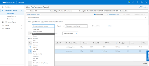
- Enhanced filtering capabilities, allowing multiple values per category, such as IP addresses, hosts, nodes, and protocols, making it easier to compare performance across multiple entities within the same time range.
- Strengthened security and operational integration with Single Sign-On (SSO) support using SAML-based authentication through Microsoft ADFS or Azure Entra ID.
- Direct, in-place upgrades from versions 6.1 and 6.2, simplifying the upgrade process for existing Scale and Simple deployments.
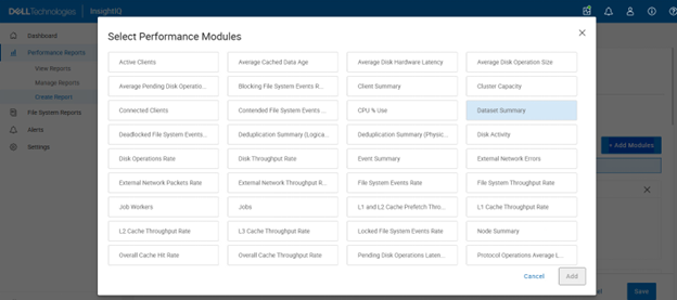
Granular Protocol Operations Breakouts
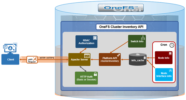
InsightIQ 6.3 introduces enhanced visibility into granular protocol-level operations through the addition of a new breakout for protocol operations. This capability is now available across all performance graphs that support operation class breakouts and includes detailed operation name breakouts for actions across both file and object, such as ‘get bucket’, ‘get object’, ‘get bucket ACL’, and related S3 operations. This is an equivalent set of operations statistics as provided by the following OneFS command:
# isi statistics pstat list --protocol s3
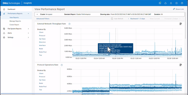
With this enhancement, users can navigate directly to performance graphs and select operation name breakouts to analyze workload behavior at a granular level. This enables identification of specific operations contributing to elevated latency or bandwidth consumption, as well as determining which operations occur most frequently. Such insights can inform operational decisions, including selectively throttling specific operations at the PowerScale layer when required.
Previously, supported graphs provided protocol-level and operation class-level breakouts. InsightIQ 6.3 extends this functionality by adding operation name-level (Op Name) visibility, allowing users to see the exact operations being executed while maintaining consistency with existing views.
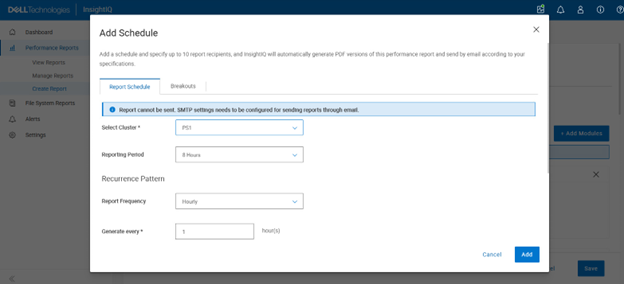
These operation name breakouts are also supported within cluster performance reports, enabling the same level of analysis in both interactive graphs and generated reports.
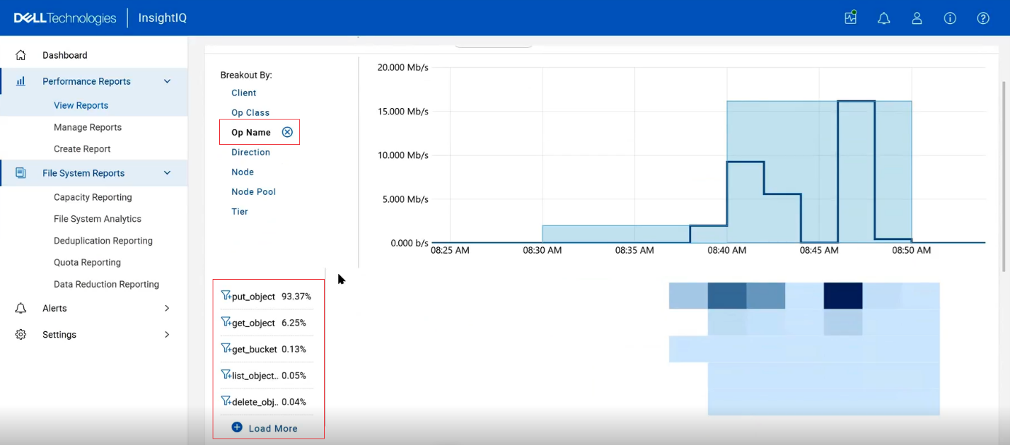
In addition, InsightIQ alerts can also now be configured using operation name (OP Name) filters with IIQ 6.3.
When defining alert rules, users may apply filters based on protocol, operation class, or specific operation names. For example, if an environment experiences a high frequency of access to a particular bucket or object, an alert can be configured specifically for the ‘get bucket’ operation to proactively notify administrators of anomalous or excessive activity.
This added granularity provides customers with significantly improved transparency into storage workloads. By exposing detailed operational metrics, including frequency, latency, and bandwidth consumption, cluster admins can more effectively identify performance bottlenecks, understand the root causes of slowdowns, and correlate workload behavior to observed performance impacts within the PowerScale cluster.
Operation names function as a subset of operation classes, which themselves are a subset of protocol performance data. This hierarchical relationship allows users to combine filters and breakouts to progressively refine analysis. For example, to analyze NFS workloads, a user may apply an NFS protocol filter and review operation class breakouts to determine whether read or write operations dominate performance time. Each operation class can then be further decomposed into individual operation names—such as specific read or object access operations—to gain deeper insight into workload behavior.
By combining protocol filters, operation class breakouts, and operation name breakouts, users can construct a highly detailed performance view that pinpoints which operations, protocols, or workload patterns contribute most significantly to latency or resource utilization.
As with existing protocol and operation class breakouts, operation name filters cannot be used in conjunction with interface-level filters. Additionally, operation name filtering is not supported with client-level filters due to limitations in OneFS telemetry data. Consequently, the system cannot report which specific client is responsible for a given operation, such as identifying which client initiated a particular ‘get object’ request.
The data presented through InsightIQ aligns with existing PowerScale CLI capabilities, such as output from the ‘isi statistics pstat list –protocol <protocol>’ command. However, while the CLI provides operation rates, InsightIQ extends this by presenting operation rates alongside bandwidth and latency metrics within a unified visualization. This delivers a more comprehensive and actionable view of protocol-level performance than was previously available through CLI data alone.
Multi-Value Breakouts
InsightIQ 6.3 introduces support for multi‑value selection within a single filter, enabling users to analyze multiple data sources simultaneously within a unified view. This enhancement allows multi‑line visualizations and aggregated insights to be presented together, simplifying side‑by‑side comparisons without requiring users to switch between views.
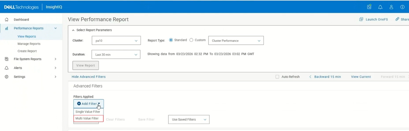
Multi‑value filter selection is supported for the following filter types: protocol, client node, node pool, and tier. For example:
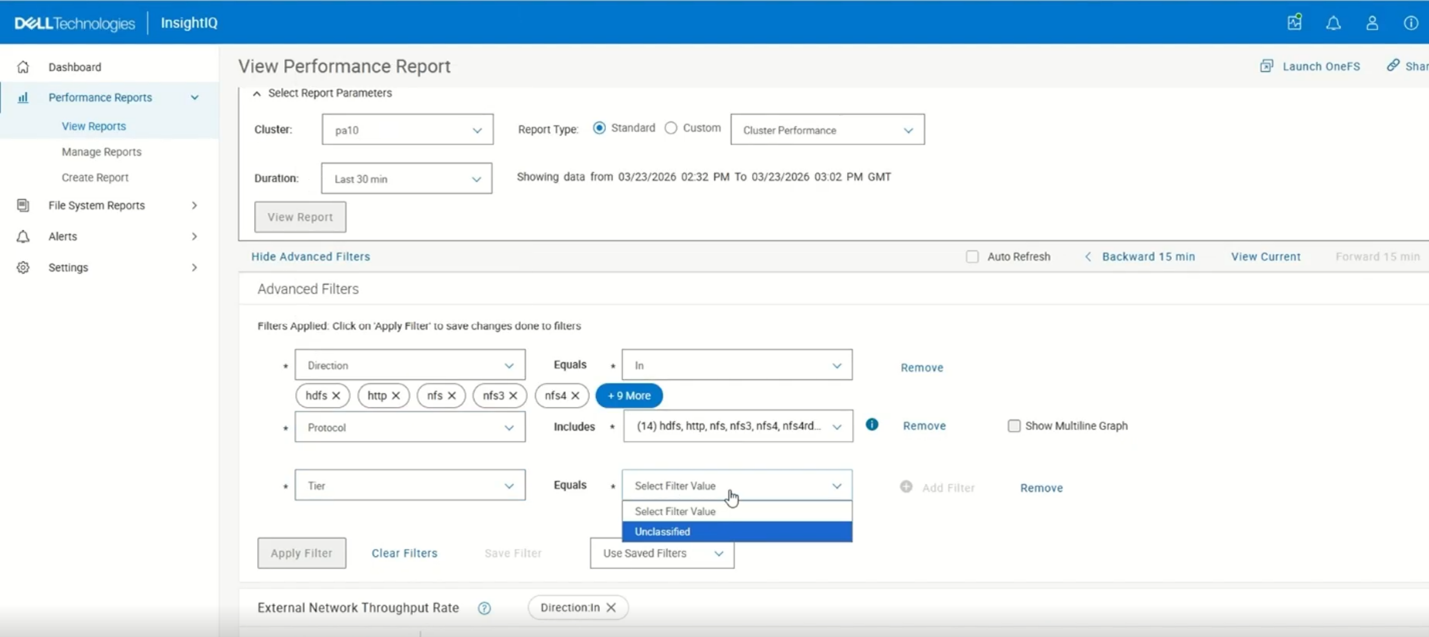
When multi‑value filtering is enabled, the ‘Breakout By’ option is automatically disabled, and the heat map view is hidden. Both features are restored when the user switches back to single‑value filter mode.
In table‑based reports, column‑level filter icons are also hidden while multi‑value filtering is active and reappear when the user reverts to single‑value selection. Download functionality supports both aggregated and multi‑value data, ensuring consistency between the UI and exported results.
When selecting multiple filter values, InsightIQ displays up to five selection ‘pills’, followed by a ‘More’ option. Selecting ‘More’ opens a pop‑up displaying all selected values, where individual entries can be removed using the corresponding remove icon. If more than five values are selected, the ‘Show Multiline Graph’ option becomes unavailable, as this feature supports only two to five filter values. Additionally, InsightIQ enforces a constraint allowing multi‑value selection on only one filter at a time; other filters must remain single‑select.
Once the filter is applied in an aggregated view, the chart presents combined metrics on a single line, with the ‘Breakout By’ option disabled and the heat map hidden.
When exporting data from this aggregated view, the resulting CSV includes a column representing the aggregate of the selected filter values, ensuring alignment between the displayed visualization and exported data.
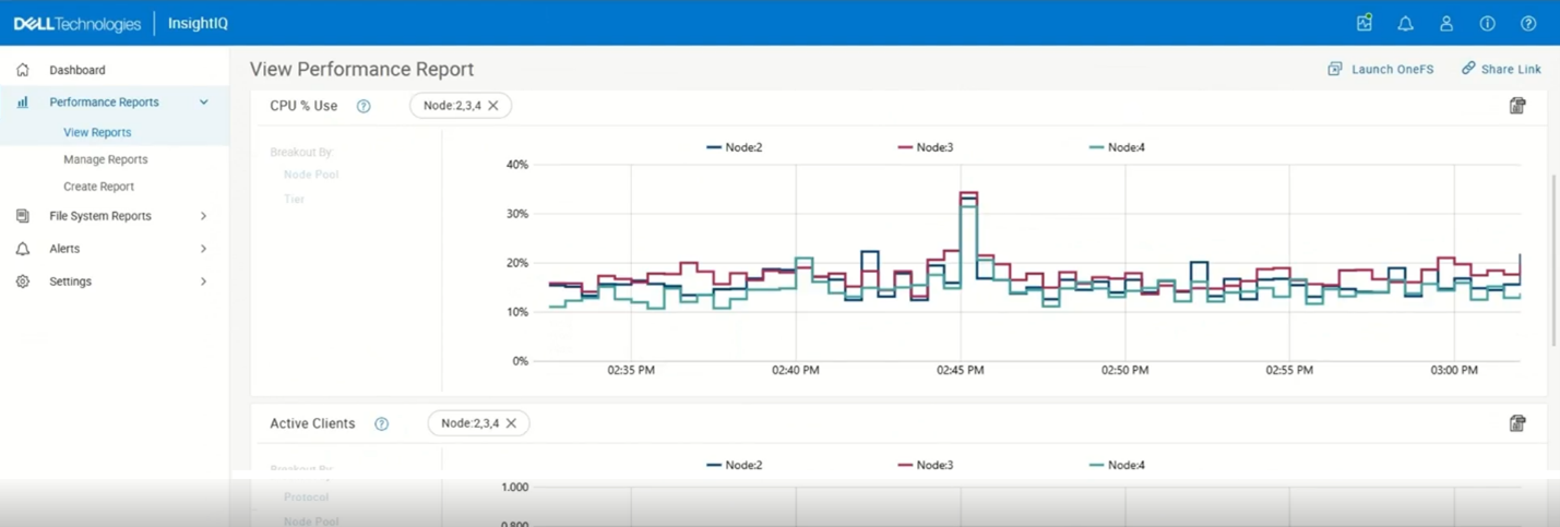
In the multi‑line scenario, users may select between two and five values (eg. multiple nodes) and enable the ‘Show Multiline Graph’ option. The resulting visualization renders a separate line for each selected value. In this mode, while the multi‑line display is preserved in the chart, the ‘Show Multiline Graph’ setting is not retained when saving filters or exporting CSV data. The exported file contains separate columns for each selected filter value, including corresponding minimum and maximum metrics, facilitating side‑by‑side comparison and offline analysis.
When viewing reports that include tabular data, such as the ‘Client Performance’ report, column‑level filter controls for attributes like address, node, and node protocol are hidden while multi‑value filtering is active. These controls are restored once the multi‑value filter is removed, allowing single‑value filtering directly from the table.
In reports where the selected filter is already part of the ‘Breakout By’ configuration (such as ‘Filesystem Cache Performance’) attempting to apply multi‑value filtering results in a notification indicating that the graph does not support this mode. This behavior is expected, as these visualizations already present multi‑line data. However, if multi‑value filtering is applied to a filter that is not used in the breakout configuration, the multi‑line chart remains available, and functions as expected.
In summary, InsightIQ 6.3 preserves the existing behavior for single‑value filtering while introducing multi‑value filtering capabilities that support both aggregated analysis and multi‑line comparisons. These enhancements provide increased analytical flexibility while maintaining consistent behavior across visualizations, reports, and exported data.
Virtual Cluster Support
InsightIQ 6.3 introduces support for monitoring virtual OneFS clusters deployed on public cloud platforms such as AWS and Azure. Historically, InsightIQ monitoring capabilities have been focused on physical PowerScale clusters. However, with the increasing adoption of cloud‑hosted virtual OneFS deployments, extending InsightIQ support to these environments has become essential.
Virtual OneFS clusters differ from physical PowerScale clusters primarily in their licensing model. While PowerScale clusters require feature‑specific licenses—such as SmartQuotas, SmartDedupe, or SmartLock—virtual OneFS clusters rely solely on a OneFS capacity license. This capacity license enables all supported OneFS features without the need for additional feature‑specific licenses.
In a physical PowerScale cluster, licensing information typically reflects multiple dynamically applied, feature‑specific licenses. By contrast, virtual OneFS clusters hosted in AWS or Azure display only the OneFS capacity license, which implicitly covers all supported features. InsightIQ 6.3 now fully understands and accounts for these licensing differences, ensuring accurate license interpretation, proper cluster type detection, and correct enablement of feature‑dependent reporting for cloud‑hosted virtual OneFS clusters.
As a result, InsightIQ now provides expanded monitoring support for customers deploying virtual OneFS clusters in public cloud environments. This enhancement ensures parity in monitoring functionality between on‑premises PowerScale clusters and cloud‑hosted virtual clusters.
| Physical OneFS cluster |
Virtual AWS/Azure based OneFS clusters |
| • Feature specific dynamic licensing (SmartQuotas, SmartDedupe etc). |
• OneFS Capacity license only
• No separate feature licenses |
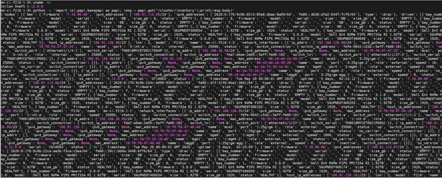
To illustrate this capability, consider a comparison of two clusters added to an InsightIQ instance. The first cluster is a standard physical PowerScale deployment. Cluster metadata obtained through CLI commands indicates that it comprises three nodes and is identified as a non‑virtual cluster. Examination of the license information shows multiple feature‑specific licenses, including SmartQuotas, SmartDedupe, and SmartLock. Certain InsightIQ reports—such as quota‑related reports—require a valid feature license to be enabled. In this case, the SmartQuotas license is active, allowing quota reports to be displayed.
The second cluster is a virtual OneFS deployment hosted in the cloud. Cluster metadata identifies it as a virtual cluster consisting of four nodes. License information for this cluster shows only the OneFS capacity license. Despite the absence of individual feature licenses, the capacity license enables full access to all supported OneFS capabilities.
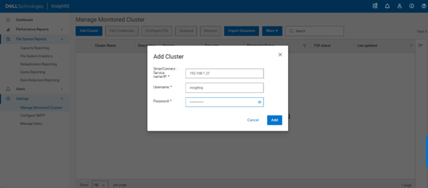
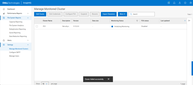
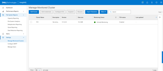
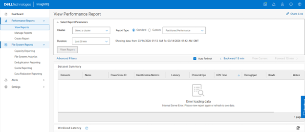
Both clusters can be added to InsightIQ using the same workflow, including credential configuration and cluster registration. Once added, InsightIQ correctly interprets the licensing model for each cluster type. For example, when viewing quota reports, InsightIQ displays the reports for the physical PowerScale cluster based on the presence of a valid SmartQuotas license. When switching to the virtual OneFS cluster, the same quota reports remain available, as the OneFS capacity license inherently enables this functionality.
With this enhancement, InsightIQ 6.3 ensures that reporting behavior remains consistent across physical and virtual deployments, regardless of underlying licensing differences. This capability significantly expands InsightIQ’s monitoring coverage, enabling comprehensive observability for both on‑premises PowerScale clusters and cloud‑hosted virtual OneFS clusters running on AWS or Azure.
SSO Support
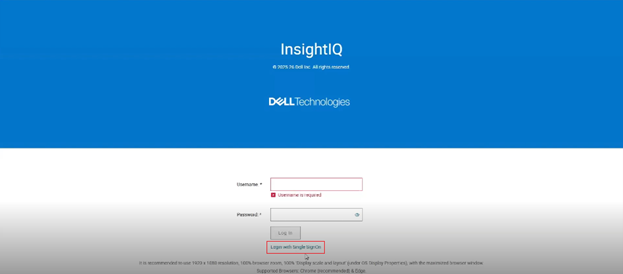
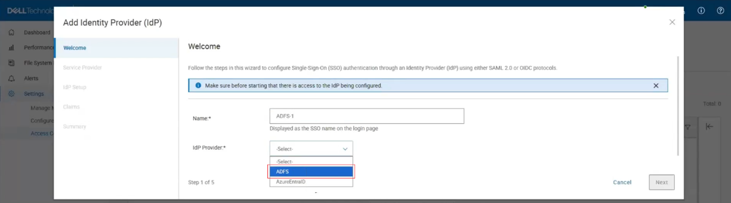
InsightIQ 6.3 introduces support for Microsoft Active Directory Federation Services (ADFS) as a new identity provider, enabling Single Sign-On (SSO) for centralized authentication and simplified access management.

In this SSO architecture, InsightIQ functions as a Service Provider (SP) and is provisioned with the required identity claims during deployment. The platform supports full lifecycle management of identity providers, allowing administrators to create, update, delete, and retrieve IdP configurations, upload ADFS federation metadata, perform test connections to validate the integration, and enable or disable the IdP through the access control interface. InsightIQ maintains a consolidated view of all provisioned identity providers along with their operational status. When at least one identity provider is enabled, an SSO login option is automatically displayed on the InsightIQ home page.
The Launch OneFS workflow has been enhanced to support SSO-based access. When a user authenticates to InsightIQ using SSO and the same SSO configuration is present on the target PowerScale cluster, selecting the ‘Launch OneFS’ option opens the PowerScale dashboard directly without additional authentication prompts.
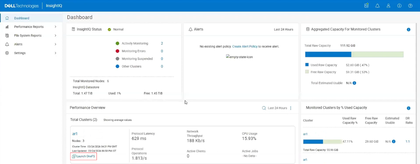
If SSO is not configured on the target cluster, the user is redirected to the PowerScale login page. This behavior change applies only to SSO-based authentication and does not affect existing local, Active Directory, or LDAP login mechanisms.
InsightIQ access control remains group-based and relies on Active Directory group membership. Active Directory administrators are responsible for assigning users from the same or trusted forests to the appropriate groups to grant InsightIQ access. The ADFS administrator must configure the identity provider to integrate correctly with an internal or external LDAP or Active Directory server so that accurate group membership information can be included in authentication claims and passed to InsightIQ for authorization decisions.
Several prerequisites must be met to enable SSO with ADFS in InsightIQ 6.3. InsightIQ version 6.3 must be installed on a supported Simple or Scale system, and the End User License Agreement must be accepted. An LDAP or Active Directory authentication provider must be configured and enabled in InsightIQ with appropriate group and role mappings defined. Windows Active Directory and DNS infrastructure must be properly configured and operational. Additionally, ADFS must be configured and synchronized with the same LDAP or Active Directory service used by InsightIQ to ensure consistent user and group resolution. Any mismatch in directory configuration between InsightIQ and ADFS can result in SSO authentication failures.
Single Sign-On (SSO) support using Azure EntraID is also added in InsightIQ 6.3 as a new identity provider option, enabling centralized authentication and streamlined access management in PowerScale for Azure Cloud deployments.
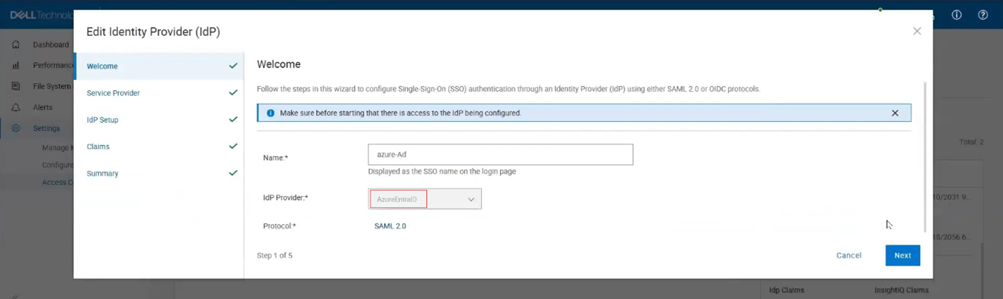
In this configuration, InsightIQ functions as a Service Provider (SP) and is provisioned with the required identity claims during deployment. The platform supports full lifecycle management of identity provider configurations, allowing administrators to create, update, delete, and retrieve IdP definitions, upload Azure EntraID federation metadata, and validate the integration through test connections. Identity providers can be enabled or disabled through the access control interface, and InsightIQ displays all provisioned IdPs along with their current status. When at least one identity provider is enabled, an SSO login option is automatically displayed on the InsightIQ home page. As part of this release, Azure EntraID is available as a newly introduced IdP type during identity provider configuration.
Several prerequisites must be satisfied to enable SSO integration with Azure EntraID. InsightIQ version 6.3 must be installed on a supported Simple or Scale system, and the End User License Agreement must be accepted. An LDAP or Active Directory authentication provider must be configured and enabled in InsightIQ, with appropriate group and role mappings defined. Windows Active Directory and DNS infrastructure must be properly configured and operational. Additionally, Azure EntraID must be configured and synchronized with the same LDAP or Active Directory service that is configured in InsightIQ to ensure accurate user and group synchronization for authentication and authorization.
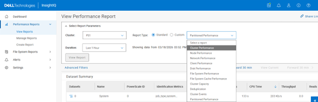
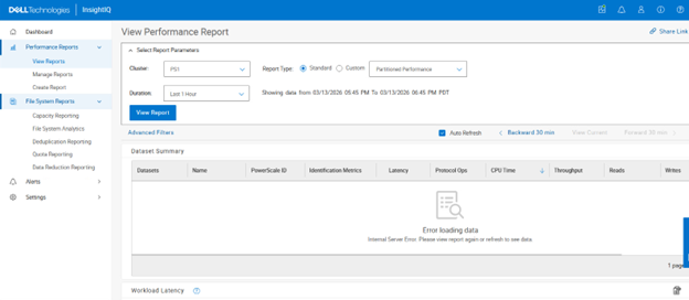
Partitioned Performance Alignment
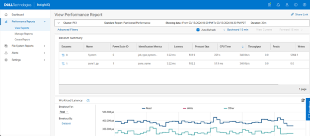
InsightIQ has aligned its partition-level performance aggregation logic with PowerScale’s native workload summary calculations. Previously, certain performance graphs in InsightIQ displayed values derived using methods that differed from those used by OneFS CLI tools or the native PowerScale UI, which could result in discrepancies when customers compared InsightIQ metrics with cluster-reported values.
With this update, non-latency metrics, such as IOPS, throughput, CPU reads, and CPU writes, are now computed using the same methodology as OneFS. As a result, InsightIQ metrics closely match those reported directly by the cluster. Latency metrics were already consistent with PowerScale calculations and remain unchanged.
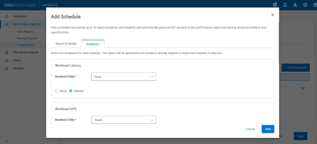
Additionally, a naming update has been introduced in InsightIQ 6.3 to improve clarity. The ‘Workload IOPS’ graph has been renamed to ‘Workload IO Operations’ to more accurately reflect the data represented by the visualization. This change is limited to labeling and does not affect underlying functionality or calculations.
From a support perspective, this enhancement directly addresses previous customer reports regarding inconsistencies between InsightIQ metrics and PowerScale cluster statistics. With the updated aggregation logic, InsightIQ graphs should now closely align with native PowerScale reporting, reducing confusion and improving confidence in performance analysis.
So, in summary, InsightIQ 6.3 offers the following attributes and functionality:
| Function |
Attribute |
Description |
| Scope |
Monitoring scope |
Up to 20 clusters and 504 nodes |
| Ecosystem |
OS support |
RHEL 8.10, RHEL 9.4, RHEL 10.0, and SLES 15 SP4 |
| Platform |
Resources |
Reduced CPUs, memory and disk requirement |
| |
|
Scale option requires just one node |
| |
Size |
Smaller package size: OVA package < 5GB |
| Install and upgrade |
Installation |
Installation time: < 12 mins |
| |
Migration |
Direct migration from 4.x |
| |
|
Online migration from InsightIQ 6.3 Simple (OVA) to InsightIQ 6.3 Scale |
| Resilience |
Data collection |
Resilient data collection – no data loss |
| OS Support |
Simple ecosystem support |
InsightIQ Simple 6.3 can be deployed on the following platforms:
· VMware virtual machine running ESXi version 8.0U3 or 9.0.1.
· VMware Workstation 17 (free version) InsightIQ Simple 6.3 can monitor PowerScale clusters running OneFS versions 9.7 through 9.14.
· OpenStack RHOSP 21 with RHEL 9.6 |
| |
Scale ecosystem support |
InsightIQ Scale 6.3 can be deployed on Red Hat Enterprise Linux versions 8.10 or 9.4 (English language versions) and SUSE Enterprise Linux (SLES) 15 SP4. InsightIQ Scale 6.3 can monitor PowerScale clusters running OneFS versions 9.7 through 9.14. |
| Upgrade |
In-place upgrade from InsightIQ 5.1.x to 6.x |
The upgrade script supports in-place upgrades from InsightIQ 5.1.x to 6.x. |
| Reporting |
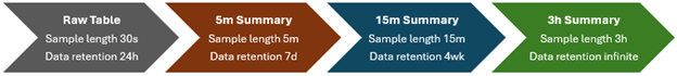
Maximum and minimum ranges on all reports |
All live Performance Reports display a light blue zone that indicates the range of values for a metric within the sample length. The light blue zone is shown regardless of whether any filter is applied. With this enhancement, users can observe trends in values on filtered graphs. |
| |
Graphing and report visualization |
Reports are designed to maximize the number of graphs that can appear on each page.
· Excess white space is eliminated.
· The report parameters section collapses when the report is run. The user can expand it manually.
· Graph heights are decreased when possible.
· Page scrolling occurs while the collapsed parameters section remains fixed at the top. |
| User interface |
What’s New dialog |
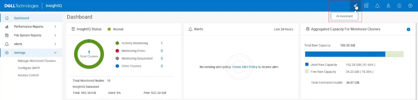
All InsightIQ users can view a brief introduction to new functionality in the latest release of InsightIQ. Access the dialog from the banner area of the InsightIQ web application. Click About > What’s New. |
| |
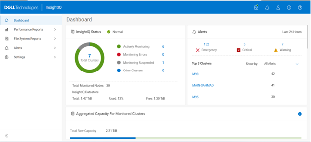
Compact cluster performance view on the Dashboard |
The IIQ dashboard provides:
· Summary information for six clusters appears in the initial dashboard view. A sectional scrollbar controls the view for additional clusters.
· The capacity section has its own scrollbar.
· The navigation side bar is collapsible into space-saving icons. Use the << icon at the bottom of the side bar to collapse it. |