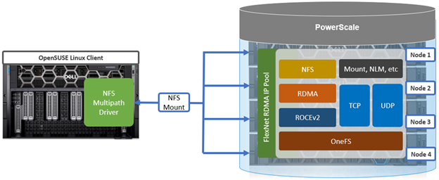
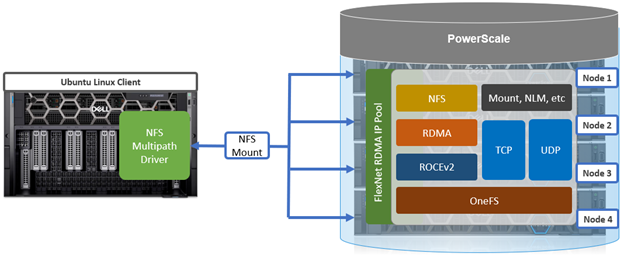
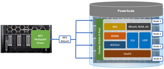
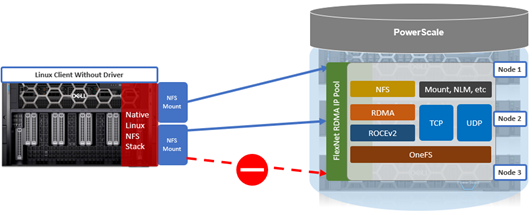
As discussed earlier in this series of articles, the multipath driver allows Linux clients to mount a PowerScale cluster’s NFS exports over NFS v3, NFS v4.1, or NFS v4.2 over RDMA.
The principal NFS mount options of interest with the multipath client driver are:
| Mount option | Description |
| nconnect | Allows the admin to specify the number of TCP connections the client can establish between itself and the NFS server. It works with remoteports to spread load across multiple target interfaces. |
| localports | Mount option that allows a client to use its multiple NICs to multiplex I/O. |
| localports_failover | Mount option allowing transports to temporarily move from local client interfaces that are unable to serve NFS connections. |
| proto | The underlying transport protocol that the NFS mount will use. Typically, either TCP or RDMA. |
| remoteports | Mount option that allows a client to target multiple servers/ NICS to multiplex I/O. Remoteports spreads the load to multiple file handles instead of taking a single file handle to avoid thrashing on locks. |
| version | The version of the NFS protocol that is to be used. The multipath driver supports NFSv3, NFSv4.1, and NFSv4.2. Note that NFSv4.0 is unsupported. |
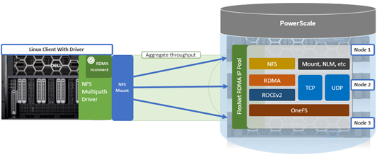
These options allow the multipath driver to be configured such that an IO stream to a single NFS mount can be spread across a number of local (client) and remote (cluster) network interfaces (ports). Nconnect allows you to specify how many socket connections you want to open to each combination of local and remote ports.
Below are some example topologies and NFS client configurations using the multipath driver.
- Here, NFSv3 with RDMA is used to spread traffic across all the front-end interfaces (remoteports) on the PowerScale cluster:
# mount -o proto=rdma,port=20049,vers=3,nconnect=18,remoteports=10.231.180.95- 10.231.180.98 10.231.180.98:/ifs/data /mnt/test
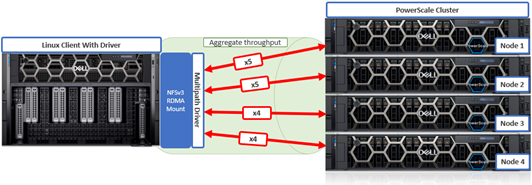
The above client NFS mount configuration would open 5 socket connections to two of the ‘remoteports’ (cluster node) IP address specified and 4 socket connections to the other two.
As you can see, this driver can be incredibly powerful given its ability to multipath comprehensively. Clearly, there are many combinations of local and remote ports and socket connections that can be configured.
- This next example uses NFSv3 with RDMA across three ‘localports’ (client) and with 8 socket connections to each:
# mount -o proto=rdma,port=20049,vers=3,nconnect=24,localports=10.219.57.225- 10.219.57.227, remoteports=10.231.180.95-10.231.180.98 10.231.180.98:/ifs/data /mnt/test

- This final config specifies NFSv4.1 with RDMA using a high connection count to target multiple nodes (remoteports) on the cluster:
# mount -t nfs –o proto=rdma,port=20049,vers=4.1,nconnect=64,remoteports=10.231.180.95- 10.231.180.98 10.231.180.98:/ifs/data /mnt/test
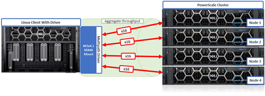
In this case, 16 socket connections will be opened to each of the four specified remote (cluster) ports for a total of 64 connections.
Note that the Dell multipath driver has a hard-coded limit of 64 nconnect socket connections per mount.
Behind the scenes, the driver uses a network map to store the local and remote port and nconnect socket configuration.
The multipath driver supports both IPv4 and IPv6 addresses for local and remote port specification. If a specified IP address is unresponsive, the driver will remove the offending address from its network map.
Note that the Dell multipath driver supports NFSv3, NFSv4.1, and NFSv4.2 but is incompatible with NFSv4.0.
On Ubuntu 20.04, for example, NFSv3 and NFSv4.1 are both fully-featured. In addition, the ‘remoteports’ behavior is more obvious with NFSv4.1 because the client state is tracked:
# mount -t nfs -o vers=4.1,nconnect=8,remoteports=10.231.180.95-10.231.180.98 10.231.180.95:/ifs /mnt/test
And from the cluster:
cluster# isi_for_array 'isi_nfs4mgmt'

ID                Vers   Conn   SessionId     Client Address Port   O-Owners      Opens  Handles L-Owners

2685351452398170437  4.1    tcp    5           10.219.57.229  872    0     0     0     0

5880148330078271256   4.1    tcp    11          10.219.57.229  680    0     0     0     0

2685351452398170437   4.1    tcp    5           10.219.57.229  872    0     0     0     0

6230063502872509892   4.1    tcp    1           10.219.57.229  895    0     0     0     0

6786883841029053972   4.1    tcp    1           10.219.57.229  756    0     0     0     0
With a single mount, the client has created many connections across the server.
This also works with RDMA:
# mount -t nfs -o vers=4.1,proto=rdma,nconnect=4 10.231.180.95:/ifs /mnt/test

# isi_for_array 'isi_nfs4mgmt’

ID                 Vers   Conn   SessionId     ClientAddress  Port   O-Owners      Opens  Handles L-Owners

6786883841029053974   4.1    rdma   2           10.219.57.229  54807  0     0     0     0

6230063502872509894   4.1    rdma   2           10.219.57.229  34194  0     0     0     0

5880148330078271258   4.1    rdma   12          10.219.57.229  43462  0     0     0     0

2685351452398170443  4.1    rdma   8           10.219.57.229  57401  0     0     0     0


0
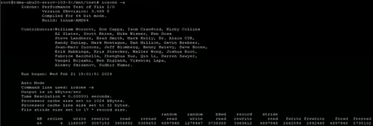
Once the Linux client NFS mounts have been configured, their correct functioning can be easily verified by generating read and/or write traffic to the PowerScale cluster and viewing the OneFS performance statistics. Running a load generator like ‘iozone’ is a useful way to generate traffic on the NFS mount. The iozone utility can be invoked with its ‘-a’ flag to select full automatic mode. This produces output that covers all tested file operations for record sizes of 4k to 16M for file sizes of 64k to 512M.
# iozone -a
For example:
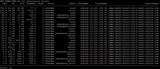
From the PowerScale cluster, if the multipath driver is working correctly the ‘isi statistics client’ CLI command output will show the Linux client connecting and generating traffic to all of the cluster’s nodes that are specified in the’ –remoteports’ option for the NFS mount.
# isi statistics client
For example:
Alternatively, from the client, the ‘netstat’ CLI command can be used from the Linux client to query the number of TCP connections established:
# netstat -an | grep 2049 | grep EST | sort -k 5
On Linux systems, the ‘netstat’ command line utility typically requires the ‘net-tools’ package to be installed.
Since NFS is a network protocol, when it comes to investigating, troubleshooting, and debugging multipath driver issues, one of the most useful and revealing troubleshooting tools is a packet capturing device or sniffer. These provide visibility into the IP packets as they are transported across the Ethernet network between the Linux client and the PowerScale cluster nodes.
Packet captures (PCAPs) of traffic between client and cluster can be filtered and analyzed by tools such as Wireshark to ensure that requests, authentication, and transmission are occurring as expected across the desired NICs.
Gathering PCAPs is best performed on the Linux client-side and on the multiple specified interfaces if the client is using the ‘–localports’ NFS mount option.
In addition to PCAPs, the following three client-side logs are another useful place to check when debugging a multipath driver issue:
| Log file | Description |
| /var/log/kern.log | Most client logging is written to this log file |
| /var/log/auth.log | Authentication logging |
| /var/log/messages | Error level message will appear here |
Verbose logging can be enabled on the Linux client with the following CLI syntax:
# sudo rpcdebug -m nfs -s all
Conversely, the following command will revert logging back to the default level:
# sudo rpcdebug -m nfs -c all
Additionally, a ‘dellnfs-ctl’ CLI tool comes packaged with the multipath driver module and is automatically available on the Linux client after the driver module installation.
The command usage syntax for the ‘dellnfs-ctl’ tool is as follows:
# dellnfs-ctl

syntax: /usr/bin/dellnfs-ctl [reload/status/trace]
Note that to operate it in trace mode, the ‘dellnfs-ctl’ tool requires the ‘trace-cmd’ package to be installed.
For example, the trace-cmd package can be installed on an Ubuntu Linux system using the ‘apt install’ package utility command:
# sudo apt install trace-cmd
The current version of the dellnfs-ctl tool, plus the associated services and kernel modules, can be queried with the following CLI command syntax:
# dellnfs-ctl status

version: 4.0.22-dell

kernel modules: sunrpc rpcrdma compat_nfs_ssc lockd nfs_acl auth_rpcgss rpcsec_gss_krb5 nfs nfsv3 nfsv4

services: rpcbind.socket rpcbind rpc-gssd rpc_pipefs: /run/rpc_pipefs
With the ‘reload’ option, the ‘dellnfs-ctl’ tool uses ‘modprobe’ to reload and restart the NFS RPC services. For example:
# dellnfs-ctl reload

dellnfs-ctl: stopping service rpcbind.socket

dellnfs-ctl: umounting fs /run/rpc_pipefs

dellnfs-ctl: unloading kmod nfsv3

dellnfs-ctl: unloading kmod nfs

dellnfs-ctl: unloading kmod nfs_acl

dellnfs-ctl: unloading kmod lockd

dellnfs-ctl: unloading kmod compat_nfs_ssc

dellnfs-ctl: unloading kmod rpcrdma

dellnfs-ctl: unloading kmod sunrpc

dellnfs-ctl: loading kmod sunrpc

dellnfs-ctl: loading kmod rpcrdma

dellnfs-ctl: loading kmod compat_nfs_ssc

dellnfs-ctl: loading kmod lockd

dellnfs-ctl: loading kmod nfs_acl

dellnfs-ctl: loading kmod nfs

dellnfs-ctl: loading kmod nfsv3

dellnfs-ctl: mounting fs /run/rpc_pipefs

dellnfs-ctl: starting service rpcbind.socket

dellnfs-ctl: starting service rpcbind
In the event that a problem is detected, it is important to run the reload script before uninstalling or reinstalling the driver. Because the script runs modprobe, the kernel modules that are modified by the driver will be reloaded.
Note that this will affect existing NFS mounts. As such, any active mounts will need to be re-mounted after a reload is performed.
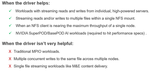
As we have seen throughout this series of articles, the core benefits of the Dell multipath driver include:
- Better single NFS mount performance.
- Increased bandwidth for single NFS mount with multiple R/W streaming files.
- Improved performance for heavily used NIC’s to a single PowerScale Node.
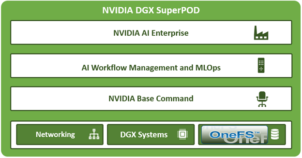
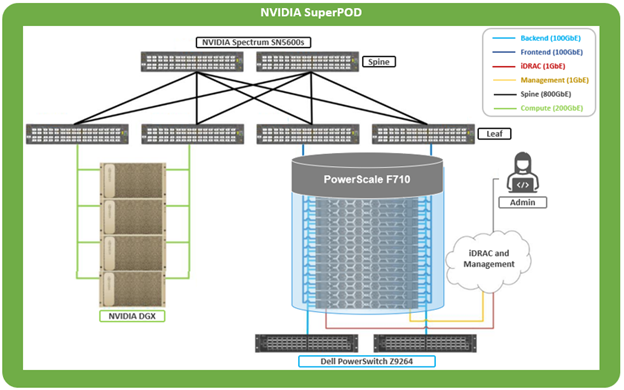
The Dell multipath driver allows NFS clients to direct I/O to multiple PowerScale nodes through a single NFS mount point for higher single-client throughput. This enables Dell to deliver the first Ethernet storage solution validated on NVIDIA’s DGX SuperPOD.