The Hadoop Distributed File System (HDFS) permissions model for files and directories has much in common with the ubiquitous POSIX model. HDFS access control lists, or ACLs, are Apache’s implementation of POSIX.1e ACLs, and each file and directory is associated with an owner and a group. The file or directory has separate permissions for the user that is the owner, for other users that are members of the group, and for all other users.
However, in addition to the traditional POSIX permissions model, HDFS also supports POSIX ACLs. ACLs are useful for implementing permission requirements that differ from the natural organizational hierarchy of users and groups. An ACL provides a way to set different permissions for specific named users or named groups, not only the file’s owner and the file’s group. HDFS ACL also support extended ACL entries, which allow multiple users and groups to configure different permissions for the same HDFS directory and files.
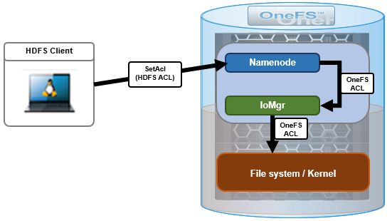
Compared to regular OneFS ACLs, HDFS ACLs differ in both structure and access check algorithm. The most significant difference is that the OneFS ACL algorithm is cumulative, so that if a user is requesting red-write-execute access, this can be granted by three different OneFS ACEs (access control entries). In contrast, HDFS ALCs have a strict, predefined ordering of ACEs for the evaluation of permissions and there is no accumulation of permission bits. As such, OneFS uses a translation algorithm to bridge this gap. For instance, here’s an example of the mappings between HDFS ACEs and OneFS ACEs:
| HDFS ACE | OneFS ACE |
| user:rw- | allow <owner-sid> std-read std-write
deny <owner-sid> std-execute |
| user:sheila:rw- | allow <owner-sheilas-sid> std-read std-write
deny <owner-shelias-sid> std-execute |
| group::r– | allow <group-sid> std-read
deny <group-sid> std-write std-execute |
| mask::rw- | posix-mask <everyone-sid> std-read std-write
deny <owner-sid> std-execute |
| other::–x | allow <everyone-sid> std-execute
deny <everyone-sid> std-read std-write |
The HDFS Mask ACEs (derived from POSIX.1e) are special access control entries which apply to every named user and group, and represent the maximum permissions that a named user or any group can have for the file. They were introduced essentially to extend traditional read-write-execute (RWX) mode bits to support the ACLs model. OneFS translates these Mask ACEs to a ‘posix-mask’ ACE, and the access checking algorithm in the kernel applies the mask permissions to all appropriate trustees.
On translation of an HDFS ACL -> OneFS ACL ->HDFS ACL, OneFS is guaranteed to return the same ACL However, translation a OneFS ACL->HDFS ACL->OneFS ACL can be unpredictable. OneFS ACLs are richer that HDFS ACLs and can lose info when translated to HDFS ACLs when dealing with HDFS ACLs with multiple named groups when a trustee is a member of multiple groups. So, for example, if a user has RWX in one group, RW in another, and R in a third group, results we be as expected and RWX access will be granted. However, if a user has W in one group, X in another, and R in a third group, in these rare cases the ACL translation algorithm will prioritize security and produce a more restrictive ‘read-only’ ACL.
Here’s the full set of ACE mappings between HDFS and OneFS internals:
| HDFS ACE permission | Apply to | OneFS Internal ACE permission |
| rwx | Directory | allow dir_gen_read, dir_gen_write, dir_gen_execute, delete_child
deny |
| File | allow file_gen_read, file_gen_write, file_gen_execute
deny |
|
| rw- | Directory | allow dir_gen_read, dir_gen_write, delete_child
deny traverse |
| File | allow file_gen_read, file_gen_write
deny execute |
|
| r-x | Directory | allow dir_gen_read, dir_gen_execute,
deny add_file, add_subdir, dir_write_ext_attr, delete_child, dir_write_attr |
| File | allow file_gen_read, file_gen_execure
deny file_write, append, file_write_ext_attr, file_write_attr |
|
| r– | Directory | allow dir_gen_read
deny add_file, add_subdir, dir_write_ext_attr, traverse, delete_child, dir_write_attr |
| File | allow file_gen_read
deny file_write, append, file_write_ext_attr, execute, file_write_attr |
|
| -wx | Directory | allow dir_gen_write, dir_gen_execute, delete_child, dir_read_attr
deny list, dir_read_ext_attr |
| File | Allow file_gen_write, file_gen_execute, file_read_attr
deny file_read, file_read_ext_attr |
|
| -w- | Directory | allow dir_gen_write, delete_child, dir_read_attr
deny list, dir_read_ext_attr, traverse |
| File | Allow file_gen_write, file_read_attr
deny file_read, file_read_ext_attr, execute |
|
| –x | Directory | allow dir_gen_execute, dir_read_attr
deny list, add_file, add_subdir, dir_read_ext_attr, dir_write_ext_attr, delete_child |
| File | allow file_gen_execute, file_read_attr
deny file_read, file_write, append, file_read_ext_attr, file_write_ext_attr, file_write_attr |
|
| — | Directory | allow std_read_dac, std_synchronize, dir_read_attr
deny list, add_file, add_subdir, dir_read_ext_attr, dir_write_ext_attr, traverse, delete_child, dir_write_attr |
| File | allow std_read_dac, std_synchronize, file_read_attr
deny file_read, file_write, append, file_read_ext_attr, file_write_ext_attr, execute, file_write_attr |
Enabling HDFS ACLs is typically performed from the OneFS CLI, and can be configured at a per multi-tenant access zone granularity. For example:
# isi hdfs settings modify --zone=System --hdfs-acl-enabled=true

# isi hdfs settings --zone=System

                  Service: Yes

       Default Block Size: 128M

    Default Checksum Type: none

      Authentication Mode: simple_only

           Root Directory: /ifs/data

          WebHDFS Enabled: Yes

            Ambari Server:

          Ambari Namenode:

              ODP Version:

     Data Transfer Cipher: none

 Ambari Metrics Collector:

         HDFS ACL Enabled: Yes

Hadoop Version 3 Or Later: Yes
Note that the ‘hadoop-version-3’ parameter should be set to ‘false’ if the HDFS client(s) are running Hadoop 2 or earlier. For example:
# isi hdfs settings modify --zone=System --hadoop-version-3-or-later=false

# isi hdfs settings --zone=System

                  Service: Yes

       Default Block Size: 128M

    Default Checksum Type: none

      Authentication Mode: simple_only

           Root Directory: /ifs/data

          WebHDFS Enabled: Yes

            Ambari Server:

          Ambari Namenode:

              ODP Version:

     Data Transfer Cipher: none

 Ambari Metrics Collector:

         HDFS ACL Enabled: Yes

Hadoop Version 3 Or Later: No
Other useful ACL configuration options include:
# isi auth settings acls modify --calcmodegroup=group_only
Specifies how to approximate group mode bits. Options include:
| Option | Description |
| group_access | Approximates group mode bits using all possible group ACEs. This causes the group permissions to appear more permissive than the actual permissions on the file. |
| group_only | Approximates group mode bits using only the ACE with the owner ID. This causes the group permissions to appear more accurate, in that you see only the permissions for a particular group and not the more permissive set. Be aware that this setting may cause access-denied problems for NFS clients, however. |
# isi auth settings acls modify --calcmode-traverse=require
Specifies whether or not traverse rights are required in order to traverse directories with existing ACLs.
# isi auth settings acls modify --group-ownerinheritance=parent
Specifies how to handle inheritance of group ownership and permissions. If you enable a setting that causes the group owner to be inherited from the creator’s primary group, you can override it on a per-folder basis by running the chmod command to set the set-gid bit. This inheritance applies only when the file is created. The following options are available:
| Option | Description |
| native | Specifies that if an ACL exists on a file, the group owner will be inherited from the file creator’s primary group. If there is no ACL, the group owner is inherited from the parent folder. |
| parent | Specifies that the group owner be inherited from the file’s parent folder. |
| creator | Specifies that the group owner be inherited from the file creator’s primary group. |
Once configured, any of these settings can then be verified with the following CLI syntax:
# isi auth setting acls view

Standard Settings

      Create Over SMB: allow

                Chmod: merge

    Chmod Inheritable: no

                Chown: owner_group_and_acl

               Access: windows

Advanced Settings

                        Rwx: retain

    Group Owner Inheritance: parent

                  Chmod 007: default

             Calcmode Owner: owner_aces

             Calcmode Group: group_only

           Synthetic Denies: remove

                     Utimes: only_owner

                   DOS Attr: deny_smb

                   Calcmode: approx

          Calcmode Traverse: require
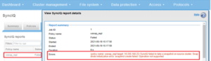
If and when it comes to troubleshooting HDFS ACLs, the /var/log/hdfs.log file can be invaluable. Setting the hdfs.log file to the ‘debug’ level will generate log entries detailing ACL and ACE parsing and configuration. This can be easily accomplished with the following CLI command:
# isi hdfs log-level modify --set debug
Here’s an example of debug level log entries showing ACL output and creation:
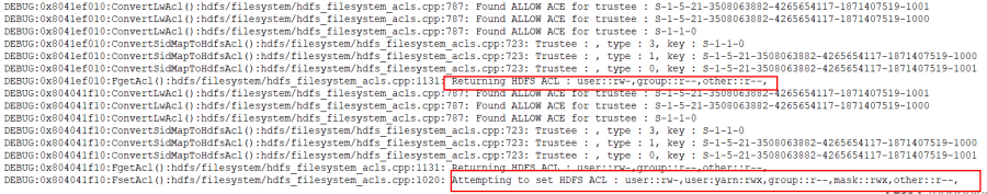
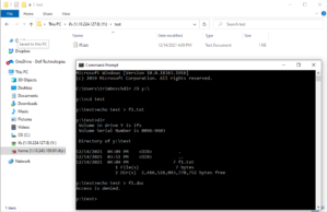
A file’s detailed security descriptor configuration can be viewed from OneFS using the ‘ls -led’ command. Specifically, the ‘-e’ argument in this command will print all the ACLs and associated ACEs. For example:
# ls -led /ifs/hdfs/file1

-rwxrwxrwx +     1 yarn  hadoop  0 Jan 26 22:38 file1

OWNER: user:yarn

GROUP: group:hadoop

0: everyone posix_mask file_gen_read,file_gen_write,file_gen_execute

1: user:yarn allow file_gen_read,file_gen_write,std_write_dac

2: group:hadoop allow std_read_dac,std_synchronize,file_read_attr

3: group:hadoop deny file_read,file_write,append,file_read_ext_attr, file_write_ext_attr,execute,file_write_attr
The access rights to a file for a specific user can also be viewed using the ‘isi auth access’ CLI command as follows:
# isi auth access --user=admin /ifs/hdfs/file1

               User

                 Name: admin

                  UID: 10

                  SID: SID:S-1-22-1-10


               File

                  Owner

                 Name: yarn

                   ID: UID:5001

                  Group

                 Name: hadoop

                   ID: GID:5000

       Effective Path: /ifs/hdfs/file1

     File Permissions: file_gen_read

        Relevant Aces: group:admin allow file_gen_read

                              Group:admin deny file_write, append,file_write_ext_attr,execute,file_wrote_attr

                              Everyone allow file_gen_read,file_gen_write,file_gen_execute

        Snapshot Path: No

          Delete Child: The parent directory allows delete_child for this user, the user may delete the file.
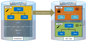
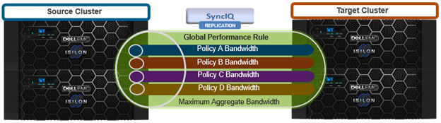
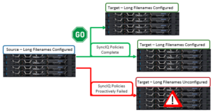
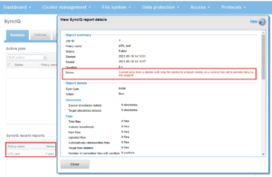
When using SyncIQ or NDMP with HDFS ACLs, be aware that replicating or restoring data from a OneFS 9.3 cluster with HDFS ACLs enabled to a target cluster running an earlier version of OneFS can result in loss of ACL detail. Specifically, the new ‘mask’ ACE type cannot be replicated or restored on target clusters running prior releases, since the ‘mask’ ACE is only introduced in 9.3. Instead, OneFS will generate two versions of the ACL – with and without ‘Mask’ – which maintains the same level of security.